The Flea Beetle Problem

This notebook is part of Bite Size Bayes, an introduction to probability and Bayesian statistics using Python.

Click here to run this notebook on Colab

import numpy as np
import pandas as pd
import matplotlib.pyplot as plt

Introduction

This notebook introduces Bayesian classification. As an example, I use data from three species of flea beetle to classify a hypothetical new specimen.

This problem is based on this data story on DASL, which is based on Lubischew, A.A. (1962), “On the use of discriminant functions in taxonomy”. Biometrics, 18, 455-477.

Different species of flea beetle can be distinguished by the width and angle of the aedeagus. The data below includes measurements and known species classification for 74 specimens.

Suppose you discover a new specimen under conditions where it is equally likely to be any of the three species. You measure the aedeagus and find width 140 microns and angle 15 (in multiples of 7.5 degrees). What is the probability that it belongs to each species?

Data

Description: Data were collected on the genus of flea beetle Chaetocnema, which contains three species: concinna (Con), heikertingeri (Hei), and heptapotamica (Hep). Measurements were made on the width and angle of the aedeagus of each beetle. The goal of the original study was to form a classification rule to distinguish the three species.

Number of cases: 74

Variable Names:

Width: The maximal width of aedeagus in the forpart (in microns)

Angle: The front angle of the aedeagus (1 unit = 7.5 degrees)

Species: Species of flea beetle from the genus Chaetocnema

We can read the data from this file:

# Load the data file
import os

if not os.path.exists('flea_beetles.csv'):
    !wget https://github.com/AllenDowney/BiteSizeBayes/raw/master/flea_beetles.csv

df = pd.read_csv('flea_beetles.csv', delimiter='\t')
df.head()

	Width	Angle	Species
0	150	15	Con
1	147	13	Con
2	144	14	Con
3	144	16	Con
4	153	13	Con

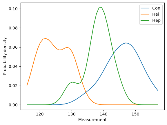
Here’s what the distributions of width look like.

def plot_cdfs(df, col):
    for name, group in df.groupby('Species'):
        cdf = Cdf(group[col], label=name)
        thinkplot.Cdf(cdf)
    
    thinkplot.decorate(xlabel=col, 
                       ylabel='CDF',
                       loc='lower right')

from scipy.stats import gaussian_kde

def plot_kdes(df, col):
    xs = np.linspace(df[col].min(), df[col].max())
    
    for name, group in df.groupby('Species'):
        kde = gaussian_kde(group[col])
        ys = kde.evaluate(xs)
        plt.plot(xs, ys, label=name)
        
    plt.xlabel('Measurement')
    plt.ylabel('Probability density')
    plt.legend()

plot_kdes(df, 'Width')

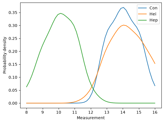
And the distributions of angle.

plot_kdes(df, 'Angle')

I’ll group the data by species and compute summary statistics.

grouped = df.groupby('Species')

Here are the means.

means = grouped.mean()
means

	Width	Angle
Species
Con	146.190476	14.095238
Hei	124.645161	14.290323
Hep	138.272727	10.090909

And the standard deviations.

stddevs = grouped.std()
stddevs

	Width	Angle
Species
Con	5.626891	0.889087
Hei	4.622758	1.101319
Hep	4.142484	0.971454

And the correlations.

for name, group in grouped:
    corr = group.Width.corr(group.Angle)
    print(name, corr)

Con -0.193701151757636
Hei -0.06420611481268004
Hep -0.12478515405529579

Those correlations are small enough that we can get an acceptable approximation by ignoring them, but we might want to come back later and write a complete solution that takes them into account.

Computing likelihoods

from scipy.stats import norm

dist_width = {}
dist_angle = {}
for name, group in grouped:
    dist_width[name] = norm(group.Width.mean(), group.Width.std())
    dist_angle[name] = norm(group.Angle.mean(), group.Angle.std())

table = pd.DataFrame()
table['hypo'] = ['Con', 'Hei', 'Hep']
table['prior'] = 1/3
table

	hypo	prior
0	Con	0.333333
1	Hei	0.333333
2	Hep	0.333333

table['likelihood'] = [dist_width[hypo].pdf(140) 
                       for hypo in table['hypo']]
table

	hypo	prior	likelihood
0	Con	0.333333	0.038709
1	Hei	0.333333	0.000347
2	Hep	0.333333	0.088287

We’ll start with equal priors

table['unnorm'] = table['prior'] * table['likelihood']
prob_data = table['unnorm'].sum()
table['posterior'] = table['unnorm'] / prob_data
table

	hypo	prior	likelihood	unnorm	posterior
0	Con	0.333333	0.038709	0.012903	0.303977
1	Hei	0.333333	0.000347	0.000116	0.002724
2	Hep	0.333333	0.088287	0.029429	0.693298

table2 = pd.DataFrame()
table2['hypo'] = table['hypo']
table2['prior'] = table['posterior']

table2['likelihood'] = [dist_angle[hypo].pdf(15) 
                       for hypo in table['hypo']]
table2

	hypo	prior	likelihood
0	Con	0.303977	0.267359
1	Hei	0.002724	0.294327
2	Hep	0.693298	0.000001

table2['unnorm'] = table2['prior'] * table2['likelihood']
prob_data = table2['unnorm'].sum()
table2['posterior'] = table2['unnorm'] / prob_data
table2

	hypo	prior	likelihood	unnorm	posterior
0	Con	0.303977	0.267359	8.127101e-02	0.99022
1	Hei	0.002724	0.294327	8.018754e-04	0.00977
2	Hep	0.693298	0.000001	8.114748e-07	0.00001

Based on these measurements, the specimen is very likely to be an example of Chaetocnema concinna.

Copyright 2020–2026 Allen Downey

Code license: MIT License

Text license: CC BY-NC-SA 4.0